Finally, Microsoft Excel brings PivotTables to iPads

Microsoft Excel for iPad has introduced full-fledged PivotTable creation and editing, expanding data analysis capabilities beyond the desktop.

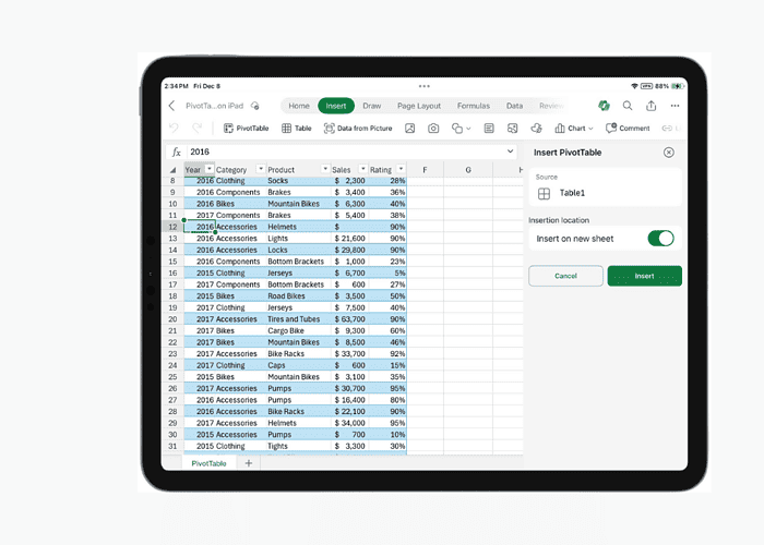
With a few taps, you can generate a PivotTable from existing data and customize it to your needs. The interface is optimized for the iPad’s touchscreen, making dragging and dropping fields a breeze.

The Field List simplifies rearranging data points across rows, columns, and filters, facilitating insightful data exploration. Moreover, the PivotTables can seamlessly adapt to updated source data through a dedicated side pane, ensuring analysis remains accurate and current.

A side pane for Settings lets users customize PivotTable formatting, calculations, and more. Users can easily relocate PivotTables across different sheets using cut-and-paste functionalities.

Here’s how to do it:

• To create a PivotTable, select PivotTable from the Insert tab and choose a source and insertion location.
• Use the field list to rearrange fields easily and tailor the PivotTable to meet your needs.
• Adjust your PivotTable’s source data seamlessly by engaging the Change Data Source side pane.
• Fine-tune your PivotTable effortlessly with the Settings side pane.
• Move your PivotTable within and across worksheets through cut and paste in the context menu.

This feature requires Excel on iPad version 2.80.1203.0 and above.

More here.